
XYOM, MISCELLANEOUS
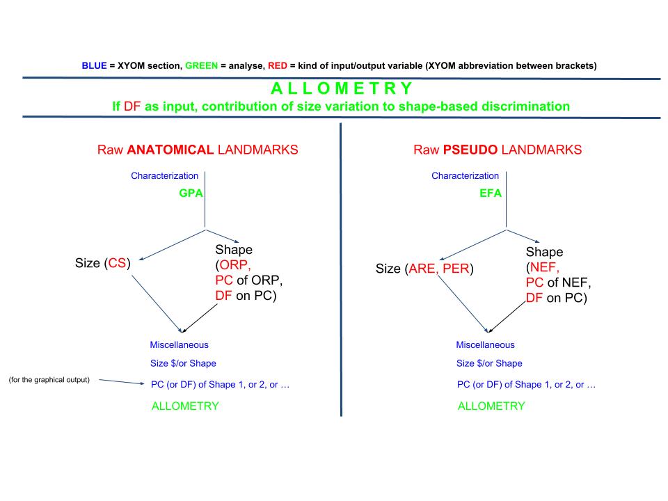
ALLOMETRY
Input (2 files): Size & Shape
Data are entered in two separate files:
- A one column file containing size (CS, PER, ARE, etc.)
- A multicolumn file containing shape (PC, or DF)
- PC or DF of tangent space variables (cfr. orthogonal projections, ORP)
- PC or DF of normalized elliptic Fourier coefficients (NEF)
- Please do not forget to indicate which column (PC, or DF, or NEF) you want to examine on the output graph.
Analyses:
The linear regression is computed (on each column of your second input file – the one containing shape data).
Output:
- Report: linear correlation coefficients, determination coefficients
- Graph: Plot of Y on X (size), with predicted values in red.
Illustration
You cannot enter raw coordinates as a “shape” file: please compute yourself the shape variables (Characterization), either ORP or NEF, and use as your second input file either their PC (first PC, generally) or the first DF in case of discriminating groups. Corresponding size data will be CS or PER/ARE, to be entered as the first input file.
COMPARISON of VARIANCES according to the Garcia (2012) method
Input (2 files): Shape & Shape
Data are characters (generally shape variables, either ORP or NEF, or their PC) from which the covariance matrices are to be compared.
You will be asked to enter two files with same number of columns (use for instance the same number of first PC of each file).
Important remark: Please be careful when it is about landmark-based shape data: they have to be computed on the concatenated files of raw coordinates and submitted to principal component analysis before to be reorganised into the two input files mentioned above.
Analyses:
For details and interpretation, please see : Garcia, C. A simple procedure for the comparison of covariance matrices BMC Evolutionary Biology 2012, 12: 222
Output:
Report,
Example:
Garcia et al. 2012: comparison of covariance matrices: Report
S1, S2 and S3 statistics are computed on the eigenvalues expressed as proportions of the total variance, and divided by 8 (the maximum for S1) so that they could vary between zero and 1.
S1 (general differentiation) is decomposed into:
S2 (difference in orientation)
and
S3 (difference in shape)
S1 0.04153369286655641
S2 0.030532958527033756
S3 0.01100073433952266
S1 5 % c. i.: from 0.03558030317506227 to 0.08834383776763419
S2 5 % c. i.: from 0.02887768619190432 to 0.07711978872395149
S3 5 % c. i.: from 0.00310489936622955 to 0.015467977480155125
Escoufier’s coefficient: COVARIATION of SHAPE of two parts of the same body (eg. head and wing)
Input (2 files): Shape & Shape
Two files, having the same number of rows (they correspond to the same individuals)
Variables are shape variables describing for each individual two (successive) different parts of the body. These shape variables have been computed separately, for example one set for the head, the other for the wings.
In both files the order of individuals must be exactly the same (the program will concatenate the two sets by columns).
Analyses:
- PLS (Partial Least Squares): silently (wait for later XYOM version to see the report)
- Escoufier’s coefficient, with confidence interval (1000 bootstraps)
Output:
Report,
Example:
Escoufier coefficient: Report
Coefficient of Escoufier 0.14687039006109312
5 % confidence interval: from 0.062087525956944535 to 0.2902682784015856
Graphical output is in preparation (PLS related graphs)
Escoufier’s coefficient: COVARIATION of SHAPE with external parameter (eg. head and latitude)
Input (2 files): Shape & Other (please use “Shape & Shape”)
WARNING: A standardisation step is necessary for external parameter data
Analyses & Output: as above
METRIC DISPARITY of landmark-based shape
Input: raw (coordinates of) landmarks
- A single file containing raw coordinates of anatomical landmarks
- Subdivision (if there is no subdivision, please enter the total number of rows)
Analyses automatically performed by XYOM:
- GPA of each group
- The sum of diagonal (trace) of variance-covariance matrix of shape variables (tangent space variables, also called Procrustes residuals or Orthogonal projections ORP) of each group.
- Bootstrap to compare group disparities according to subdivisions
(if there is no subdivision, please enter the total number of rows)
Output:
Report,
Example:
— — —
Metric Disparity, or Variance of Shape: Report
— — —
Variance of shape, group 1: 0.0017094319564931848
Variance of shape, group 2: 0.0018580320534635488
Variance of shape, group 3: 0.001345167825046605
Between group 1 and group 2: not S at P = 0.05
Between group 1 and group 3: not S at P = 0.05
Between group 2 and group 3: not S at P = 0.05
(1000 bootstraps, cfr. Zelditch et al, 2004)
METRIC DISPARITY of outline-based shape
Input: raw (coordinates of) pseudolandmarks
- raw coordinates of contours (pseudolandmarks)
- subdivision
Analyses automatically performed by XYOM::
- EFA of each group
- The sum of diagonal (trace) of variance-covariance matrix of shape variables (Normalised Elliptic Fourier coefficients, or NEF) of each group
- Bootstrap to compare group disparities according to subdivisions
(if there is no subdivision, please enter the total number of rows)
Output: as above.
REPEATABILITY
Input (2 files): Shape & Shape , Size &/orShape
The statistical method followed by XYOM for the estimation of size repeatability follows a Model II one-way ANOVA for repeated measures (G. Arnqvist, T. Mårtensson. ”Measurement error in geometric morphometrics: Empirical strategies to assess and reduce its impact on measures of shape.” Acta Zoologica Academiae Scientiarum Hungaricae, vol44, no.1-2, pp.73–96, 1998).
The statistical method followed by XYOM for the estimation of shape repeatability is the Procrustes ANOVA (Goodall, C.R. 1991. Procrustes methods in the statistical analysis of shape. Journal of the Royal Statistical Society B 53:285-339; Christian Peter Klingenberg, Grant S. McIntyre and Stefanie D. Zaklan. 1998. Left-right asymmetry of fly wings and the evolution of body axes. Proc. R. Soc. Lond. B. 265, 1255-1259)
INPUT. Two files containing the same individuals. In both files the order of individuals is exactly the same.
Variables must be shape variables computed from 2 (successive) digitisation sessions, either orthogonal projections after Procrustes superimposition (ORP), or normalised elliptic Fourier coefficients (NEF).
WARNING: for anatomical landmarks (LM), size and shape must be computed on the total sample of raw LM (the first digitisation set followed by the second one). The two input files are then extracted (or “splitted”) from the size output (if it is about size repeatability), or from the shape output (if it is about shape repeatability). Please consider the illustration below:
WARNING: for size or for shape obtained from pseudolandmarks (outlines), there is no special need to merge the raw coordinates to produce (size and) shape variables from the two digitisation sessions. The normalized elliptic Fourier coefficients (NEF, or shape variables) may be computed individually, they do not depend on the total sample parameters.
XYOM, MISCELLANEOUS: FILES UTILITIES
File Conversion
- XYOM reads the CLIC format. While the input file for XYOM must follow the CLIC format, the output file(s) may be issued in different formats: CLIC, TPS, CVS or JSON formats.
- To submit a TPS format to XYOM, you should first convert it to the CLIC format. This conversion will extract the landmarks and only the landmarks, with a very first row of free comment of your own.
- If you want to convert a TPS format to the CLIC (XYOM) format, just ask the conversion to be performed from TPS to CLIC. Please note that it is restricted to landmarks, there is no conversion from .DTA or .TPS of pseudolandmarks to the XYOM format.
- NOT IMPLEMENTED YET –> If you want to convert a TPS format to the CLIC_DB format, just ask the conversion to be performed from TPS to CLIC_DB. Then, you can extract the CLIC format from the CLIC_DB or from the TPS.
- To submit pseudolandmarks to XYOM, you must follow a special arrangement for the three first columns (number of points, x and y coordinates of the centroid point), see XYOM format.
- It is possible to convert a table of pseudolandmarks to the CLIC OTL format.
Selecting columns from a given file
Please enter the first and last columns of the sub-matrix to be extracted
A new file is created corresponding to the range of columns you indicated.
Selecting rows from a given file
Please enter the first and last rows of the sub-matrix to be extracted
A new file is created corresponding to the range of rows you indicated.
Concatenating files by rows
Input: 2 files, same number of columns (or not if they are outlines files)
Output: A new file is created merging the two files by rows
Concatenating files by columns
Input: 2 files, same number of rows
Output: A new file is created merging the two files by clolumns